Pong from Pixels.

Starting where the field started.

Deep reinforcement learning has a clear origin point. In 2013, DeepMind published a network that learned to play Atari games directly from the pixels of the screen, using deep Q-learning; the 2015 follow-up in Nature showed it reaching human-level play across many of those games. Pong was one of them. It was the first time a single architecture learned control from raw images at that scale.

That result is the root of a lineage. The same lab went on to AlphaGo, then AlphaZero, then AlphaFold — work that reshaped its fields. You don’t need a novel idea to learn from the most important one; you need to rebuild it and watch it work. Reproducing Pong-from-pixels is a deliberate choice to begin a deep-RL education at the beginning of deep RL.

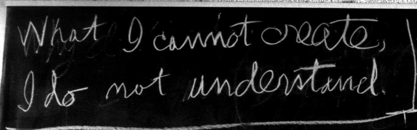
This is an homage and a reproduction, not a claim of novelty or any affiliation — the goal is understanding earned by construction. It’s the idea that was still on Richard Feynman’s blackboard when he died, and one of the convictions this project is built around.

Build the parts that teach. Import the parts that don’t.

The fastest way to learn deep RL is also the least honest: import a library, call agent.train(), and watch a number go up. The slowest is to write the GPU kernels yourself. Neither teaches the right thing. So the line is drawn deliberately — the conceptual core is hand-written, and the commodity machinery underneath is imported and named as such.

From 210×160 pixels to a move.

Each Atari frame arrives as a 210×160 colour image. It’s converted to grayscale, downsampled to 84×84, and the last four frames are stacked so the network can see motion — which way the ball is travelling, and how fast. That stack is the only input. There is no score feed, no ball coordinates, no hand-built features.

A small convolutional network maps that 84×84×4 stack to one value per action — the expected return, or Q-value, of moving up, staying, or moving down. The agent mostly takes the highest-value action and occasionally explores at random. Each transition is stored; minibatches are replayed to break correlation; and a slowly-updated copy of the network (the target network) provides a stable learning signal:

The whole thing has to fit and train on a single RTX 2060 with 6 GB of memory, which shapes everything downstream — the replay buffer size, the batch size, and how long a run realistically takes.

Four-hour Saturdays, floor and aspiration.

The project runs on a fixed cadence: one four-hour block a week. Each session is pre-registered with two targets written down before it starts — a floor (what must be true by the end) and an aspiration (the stretch). Writing both down in advance is the point: a missed aspiration isn’t failure, it’s information about where the estimate was wrong.

Three of the five phases are done — kickoff, architecture, and the core build (network, replay buffer, agent, and training loop, all assembled and running). The next phase is training and diagnosis: getting it to actually converge, and being honest about what that takes. Shipping the finished page is the last.

Get it to convergence — then tell the truth about how.

• Train the agent until it reliably beats the built-in opponent, on the 6 GB card.
• Log per-episode reward to disk, so the real learning curve replaces the representative one.
• Checkpoint the model at milestones — random, first rally, breakthrough, trained — and record a short gameplay clip at each, so the demo’s slider scrubs through real footage.
• Instrument the internals: Q-value drift, the ε schedule, replay dynamics, plus wall-clock, VRAM, and GPU temperature per run.
• Write up what actually worked and what didn’t — including the dead ends, which are the part most write-ups quietly drop.